Machine-Learning

Variational Auto Encoder

01 Sep 2022

Table of Contents

Understanding the VAE

Motivation

Generative models like the autoencoder only replicates the inputs but do not modify them in any way.
For instance, we might hope to make our model learn from images of faces with glasses and then generate similar unseen images of faces with glasses.
VAE sovles this problem by introducing randomness into the latent variable, that is, instead of learning a fixed latent vector as in the autoencoder, it learns a probability distribution.
Here is a sample generated by a VAE (source)

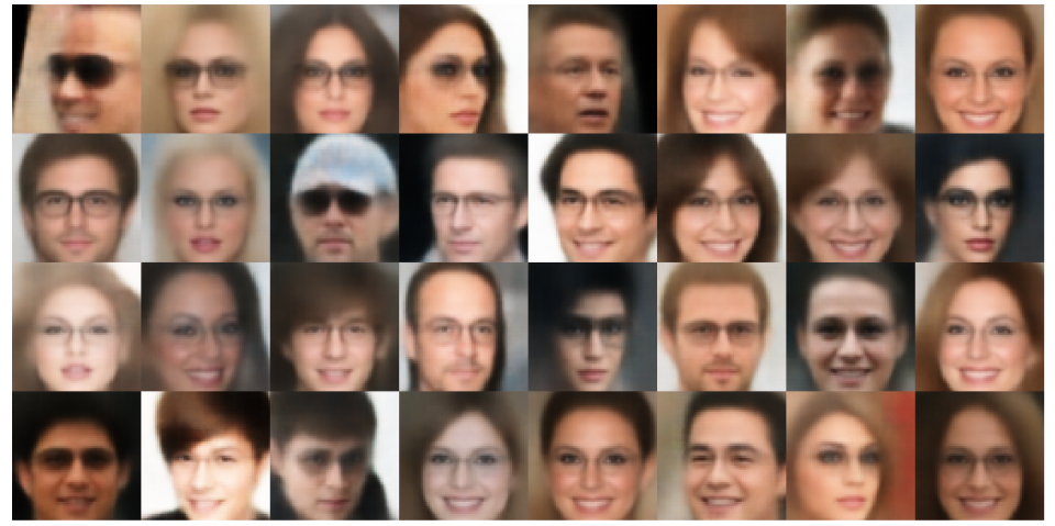
Figure 1: A VAE generating faces with glasses

Formulation

We outline the goals and define some notations.

We would like to model the distribution $P_{\theta}$ of some data $X \sim P_{\theta}$
We have a latent variable $Z$
Conditional distribution depending on $Z$ given by $P_{\theta}(X \mid Z)$ with $\theta$ being a parameter
We can view this conditional distribution as the generation process
Thus $\theta$ is called the generative model parameter
To make computation easier, we can choose a custom parametrised distribution $Q_{\phi}(Z)$ for $Z$ in order to approximate the true distribution
$\phi$ is called the variational parameter
$Q_{\phi}(Z \mid X)$ can be viewed as an encoding process [1]
Both $P$ and $Q$ can be seen as some neural networks

We take input $X$, pass it through $Q$, encodes it into some distribution, sample from the distribution, and pass it through $P$.

We describe the distribution of $X$ as follows (using marginal density):

\[p_{\theta}(x) = \int p_{\theta}(x|z) p_{\theta}(z) dz\]

For instance, we can sample $z$ from the latent distribution as a normal distribution and its parameters are learnt by the encoder. An illustration is presented below (source)

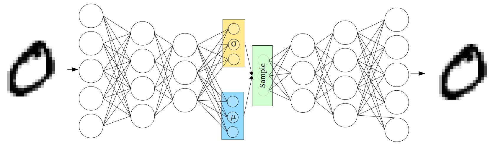
Figure 2: A VAE which encodes into mean and varianace

To choose the optimal parameters, we would like to maximise the marginal likelihood of $X$, as maximising directly is hard, we maximize the Evidence Lower Bound(ELBO)

\[\begin{aligned} \log p_\theta({x}) &\ge \mathbb{E}_{q_\phi({z}\mid{x})} \left[ \log p_\theta({x}\mid{z})\right] - D_{KL}\left( Q_\phi({z}\mid{x}) || P_\theta({z}) \right)\\ &=: -\mathcal{L}(\theta, \phi; {x}), \end{aligned}\]

where $D_{KL}$ is the Kullback-Leibler divergence between our chosen variational distribution and the true posterior distribution, defined as

\[D_{KL}\left( Q_\phi({z}\mid{x}) || P_\theta({z}) \right) = \int q_\phi({z}\mid{x})\log\left(\frac{q_\phi({z}\mid{x})}{p_\theta({z})}\right)d{z}.\]

Note that the KL-divergence can be seen as the expectation $\mathbb{E}[\log\left(\frac{q_\phi({z}\mid{x})}{p_\theta({z})}\right)]$ w.r.t. the first distribution of the difference in logs between the two distribution; it acts as a regularizer which constraint our approximate distribution $Q_{\phi}$, keeping it close to the true posterior.

We leave the derivations to the end.

Training

To train the network, we need to compute the ELBO in some way, either analytically or through MCMC sampling, then we perform some kind of gradient descent to update both $\theta$ and $\phi$.

First we compute the loss,

\[-\mathbb{E}_{q_\phi({z}\mid{x})} \left[ \log P_\theta({x}\mid{z})\right] + D_{KL}\left( Q_\phi({z}\mid{x}) || P_\theta({z}) \right)\]

We can approximate this using conditional probability to arrive at the Stochastic Gradient Variational Bayes (SGVB) estimator using Monte Carlo simulations of batch size $L$

\[\mathcal{\hat{L}}(\theta, \phi; x)= \frac{1}{L} \sum_{j=1}^L -\log p_\theta(x,z^{(j)})+ \log q_\phi(z^{(j)}|x)\]

since $\frac{p_\theta(x,z^{(j)})}{p_{\theta}(z^{(j)})}=p_{\theta}(x \mid z)$

We need to use a reparametrization trick to use gradient descent, as $z$ is sampled from a distribution. Namely, we find a continous invertible transformation $g_{\phi}(\epsilon^{(j)},x)$ mapping from a variable sampled from a fixed distribution to $z^{(j)}$, thus we arrive at the following using change of variables

\[q_{\phi}(z|x) = |\frac{d\epsilon}{dz}|p(\epsilon)\]

An example is the shift and scale of the normal distribution $z = \sigma \epsilon + \mu$.

If both $P,Q$ are normal distributions, then their KL-divergence can be computed analytically using mean and variance, in this case, we only need to sample for the first term in the loss

\[\hat{\mathcal{L}}^B(\theta,\phi;x) := \frac{1}{L} \sum_{j=1}^L -\log p_\theta(x\mid z^{(j)}) + D_{KL}(Q_\phi(z\mid x) || P_\theta(z))\]

Summary

The algorithm inputs are the encoder and decoder networks $Q_\phi(z \mid x)$, $P_\theta(x \mid z)$, prior distribution $P_\theta(z)$, minibatch size $M$ and number of Monte Carlo samples $L$.

WHILE not converged:

Sample minibatch $\mathcal{D}_m$ of $M$ data examples
Sample $M\times L$ noise variables $\epsilon^{(i, j)}$ for each $x_i\in\mathcal{D}_m$ and $1\leq j \leq L$
Compute gradient
\[\frac{1}{M}\sum_{x_i \in \mathcal{D}_m}\nabla_{\phi, \theta} \mathcal{\hat{L}}(\theta,\phi;x_i)\]
Update parameters $\theta$ and $\phi$ using SGD

Proofs

An intuitive way to derive the ELBO is to consider the KL-divergence between $Q_\phi(z\mid x)$ and $P_\theta(z\mid x)$.

\[\begin{aligned} D_{KL}(Q_\phi({z}\mid {x}) || P_\theta( {z}\mid {x})) &= \int q_\phi({z}\mid {x}) \log\left(\frac{q_\phi({z}\mid {x})}{p_\theta({z}\mid {x})}\right) d{z}\\ &= \int q_\phi({z}\mid {x}) \log\left( \frac{q_\phi({z}\mid {x})}{p_\theta({x}\mid{z})p_\theta({z}) / p_{\theta}(x)}\right) d{z}\\ &= \int q_\phi({z}\mid {x}) \log p_\theta({x}) d{z} - \int q_\phi({z}\mid{x}) \log p_\theta({x}\mid{z})d{z}\\ & \quad + \int q_\phi({z}\mid {x})\log\left( \frac{q_\phi({z}\mid {x})}{p_\theta({z})} \right)d{z}\\ &= \log p_\theta(x)-\mathbb{E}_{q_\phi({z}\mid{x})} \left[ \log P_\theta({x}\mid{z})\right] + D_{KL}\left( Q_\phi({z}\mid{x}) || P_\theta({z}) \right) \\ &= \log p_\theta({x}) + \mathcal{L}(\theta, \phi; {x}) \end{aligned}\]

which implies

\[\log p_\theta({x}) \geq -\mathcal{L}(\theta, \phi; {x})\]

as the KL-divergence is nonnegative.

References

[1] Kristiadi A. (2016) Variational Autoencoder: Intuition and Implementation

[2] Kingma, D.P., & Welling, M. (2014). Auto-Encoding Variational Bayes. CoRR, abs/1312.6114.