Brief Recap of Discrete Time Martingales 1

Table of Contents

This is a brief recap of discrete time martingales. I am using Jean Francois Le Gall’s book and David Williams’ books as references.

Update (September 2024): added more details and formatting.

Preliminaries

As usual, we set a sequence of sigma algebras $\mathcal{F}_0 \subset \mathcal{F}_1 \subset \cdots \subset \mathcal{F}_n \subset \cdots \subset \mathcal{A}$ and a sequence of random variables $(X_n)_n$ defined on a probability space $(\Omega, \mathcal{F}, P)$. We also assume that $X_n$ is $\mathcal{F}_n$-measurable for all $n$ (it’s adapted to the filtration).

Definition: A sequence of random variables $(X_n)_n$ is a martingale if for all $n$, $\mathbb{E}[|X_n|] < \infty$ and $\mathbb{E}[X_{n+1} | \mathcal{F}_n] = X_n$ a.s.

Remark: In the discrete case, we do not have to specify the conditional expectation at any time, as we can just use induction.

A simple and important case of a martingale is $X_n = \mathbb{E}[X \mid \mathcal{F}_n]$, where $X$ is a random variable. This is a closed martingale.

Similarly, we have the following definition for a submartingale and a supermartingale.

• Submartingale: $(X_n)$ is integrable and $\mathbb{E}[X_{n+1} \mid \mathcal{F}_n]\geq X_n$ a.s.
• Supermartingale: $(X_n)$ is integrable and $\mathbb{E}[X_{n+1} \mid \mathcal{F}_n] \leq X_n$ a.s.

Stopping Times

A random variable $T: \Omega \to \mathbb{N} \cup \{\infty\}$ is a stopping time if $\{T \leq n\} \in \mathcal{F}_n$ for all $n$.

In the discrete case, this is equivalent to saying that $\{T = n\} \in \mathcal{F}_n$ for all $n$. As an example, consider $T_A = \inf \{n \geq 0 : X_n \in A\}$ with $X_n$ being an adapted process and $A$ a fixed measurable set, then $\{T_A = n\} = \bigcap_{i=0}^{n-1} \{X_i \notin A\} \cap \{X_n \in A\} \in \mathcal{F}_n$

The $\sigma-$algebra of the past up to a stopping time $T$ is defined as:

\[\mathcal{F}_T = \{A \in \mathcal{F} : A \cap \{T \leq n\} \in \mathcal{F}_n \text{ for all } n\}\]

Some properties of this past sigma field are:

• $\mathcal{F}_T$ is a sigma algebra

• $\mathcal{F}_S \subset \mathcal{F}_T$ if $S \leq T$

• $\mathcal{F}_{S \wedge T} = \mathcal{F}_S \cap \mathcal{F}_T$

Remark: The last property is useful in the case where we have two stopping times, and we want to consider the past up to the first time that either of them occurs.

A random variable with subscript $T$ is defined as:

\[X_T(\omega) = X_{T(\omega)}(\omega),\]

which is $\mathcal{F}_T$-measurable.

Remark: To see this, it suffices to show that $\{X_T \in B\} \cap \{T=n\} \in \mathcal{F}_n$ for all $n$ and $B \in \mathcal{B}(\mathbb{R})$. But this the same as $\{X_n \in B\} \cap \{T=n\} \in \mathcal{F}_n$ which is true by definition of stopping time.

A common trick is to consider a stopped process

\[X_{T \wedge n}(\omega) = X_{\min(T(\omega), n)}(\omega)\]

Remark: This is useful in the case where we have some unbounded process, and we want to stop it at some time $T$. For example, if $X_n$ is a random walk, then $X_{T \wedge n}$ is a bounded random walk, with $T$ being the first time that the random walk hits some level.

Optional Stopping Theorem ver. 1

In fact, the Optional Stopping Theorem allows us to treat the stopped process as a martingale.

Optional Stopping Theorem: Let $(X_n)_n$ be a martingale and $T$ be a stopping time. Then $(X_{T \wedge n})_n$ is a martingale. In particular, if $T< \infty$, then $\mathbb{E}[X_T] = \mathbb{E}[X_0]$.

Remark: This really says that we can stop a martingale at any time, and the expectation will be the same as the initial value. So if a game is a martingale, nothing can be gained by stopping play based on the information obtainable so far.

To show this, we need the following:

Definition: A sequence of random variables $(H_n)_n$ is predictable if $H_n$ is bounded and $\mathcal{F}_{n-1}$-measurable for all $n$.

Lemma (Martingale Transform): Let $(X_n)_{n}$ be an adapted process and $(H_n)_{n}$ be a predictable process. We define $(H\cdot X)_{0}=0$ and $(H\cdot X)_{n} = \sum_{i=1}^n H_i(X_i - X_{i-1})$. Then:

• $(X_n)_{n}$ is a martingale $\implies$ $(H\cdot X)_n$ is a martingale
• $(X_n)_{n}$ is a super/submartingale $\implies$ $(H\cdot X)_{n}$ is a super/submartingale when $H_n \geq 0$ for all $n$.

Remark: Note how this is similar to the stochastic integral; the name “martingale transform” is taken from William’s book.

Remark: There is also a nice example in Durrett’s book viewing $H$ as a gambling system and $X_i-X_{i-1}$ as the change in wealth. (e.g. $H_0=1$ and then $H_i=2H_{i-1}$ if lost, while $H_i=H_{i-1}$ if won last time, so always double down if you lose)

Then to show the optional stopping theorem, we define $H_n = \mathbf{1}_{\{T\geq n\}}= 1 - \mathbf{1}_{\{T\leq n-1\}}$, which is predictable. Then

\[X_{T \wedge n} = \sum_{i=1}^{n\wedge T} H_i(X_i - X_{i-1}) + X_0 = (H\cdot X)_{n} + X_0\]

is a martingale, and so $\mathbb{E}[X_T] = \mathbb{E}[X_{T\wedge N}] = \mathbb{E}[X_0]$ for a bounded stopping time $T \leq N$, as $X_{T\wedge N}$ is a martingale from the lemma and the expectation $\mathbb{E}[(H\cdot X)_n]$ is zero.

If the stopping time is only finite almost surely, the equality will not hold, as shown in the following example.

Example: Consider a random walk $X_n = \sum_{i=1}^n \xi_i$ where $\xi_i$ are iid Radmacher with $\mathbb{P}(\xi_i = 1) = \mathbb{P}(\xi_i = -1) = \frac{1}{2}$. Let $T = \inf \{n \geq 0 : X_n = 1\}$. Then $T < \infty \ a.s.$ is a stopping time, and $\mathbb{E}[X_T] = 1$ but $\mathbb{E}[X_0] = 0$.

Martingale Convergence Theorems

Intuitively, a deterministic sequence $X_n$ converges when its “fluctuations” vanish. Controlling one direction of “fluctuations” (e.g $\sup |X_n|$) can give a subsequential limit, while controlling both directions of “fluctuations” (e.g the classical $\limsup=\liminf$) can give a limit of the sequence. So we either try to bound it or we show the equality of limits directly. It turns out that the same ideas applies to martingales.

Convergence in $L^1$

As discussed in the beginning of this section, we would like to bound the fluctuations of the martingale sequence. To do this, we introduce the concept of upcrossings.

The picture below is from Williams’ book. The strategy of playing is to wait for $X$ to dip below $a$ and start playing until it reaches $b$. The largest $k$ such that we can find times $0\leq s_1 < t_1 < s_2 < t_2 < \cdots < s_k < t_k \leq n$ with $X_{s_i} \leq a$ and $X_{t_i} \geq b$ is the number of upcrossings.

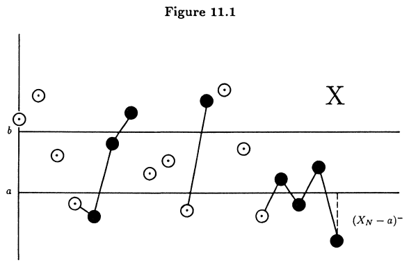
More precisely, we fix $a,b\in \mathbb{R}$ and a sequence $\alpha\subseteq \mathbb{R}$, we define two increasing sequences as the times of upcrossings:

\[\begin{aligned} S_{1}(\alpha)&:=\operatorname*{inf}\{n\geq0: \alpha_{n}\leq a\}\\ T_{1}(\alpha)&:=\operatorname*{inf}\{n\geq S_{1}(\alpha):\alpha_{n}\geq b\} \end{aligned}\]

Inductively, we have:

\[\begin{aligned} S_{k+1}(\alpha)&:=\operatorname*{inf}\{n\geq T_k(\alpha): \alpha_{n}\leq a\}\\ T_{k+1}(\alpha)&:=\operatorname*{inf}\{n\geq S_{k+1}(\alpha):\alpha_{n}\geq b\} \end{aligned}\]

where we use the convention of $\inf \emptyset = \infty$.

Here $S_i$’s are the times when the sequence dips below $a$ and $T_i$’s are the times when the sequence goes above $b$.

Then the upcrossing number for interval $[a,b]$ is:

\[\begin{aligned} N_{n}([a,b],\alpha)&=\operatorname*{sup}\{k\geq1:T_{k}(\alpha)\leq n\}=\sum_{k=1}^{\infty}\mathbf{1}_{\{T_{k}(\alpha)\leq n\}}\\ N_{\infty}([a,b],\alpha)&=\operatorname*{sup}\{k\geq1:T_{k}(\alpha)<\infty\}=\sum_{k=1}^{\infty}{\mathbf{1}}_{\{T_{k}(\alpha)<\infty\}}, \end{aligned}\]

This leads to the following analytic result which characterizes convergence of a sequence in the extended real numbers $\overline{\mathbb{R}}$.

Lemma: The sequence $(\alpha_n)_n$ converges in the extended real numbers if and only if, $\forall a,b \in \mathbb{Q}$ with $a<b$, we have $N([a,b], \alpha) < \infty$.

A proof can be found here, which uses the fact that a sequence converges iff it has $\liminf=\limsup$.

Extending this to a martingale $(X_n)_n$, we see both $S_k(X)$ and $T_k(X)$ are stopping times e.g. we can write the event $\{T_k(X)\leq n\}$ as

\[\operatorname*{\bigcup}_{0\le m_{1}<n_{1}<\dots<m_{k}<n_{k}\le n}\{X_{m_{1}}\le a,X_{n_{1}}\ge b,\dots,X_{m_{k}}\le a,X_{n_{k}}\ge b\}\]

so it’s in $\mathcal{F}_n$; a similar formula holds for $S_k(X)$.

As a result, $N_\infty([a,b], X)$ is also $\mathcal{F}_n$ measurable. To bound this random variable, we have the following lemma.

Doob's Upcrossing Inequality: Let $(X_n)_n$ be a submartingale. Then for all $a<b$ and every $n\in \mathbb{N}$, $$ (b-a)\,\mathbb{E}[N_{n}([a,b],X)]\leq\mathbb{E}[(X_{n}-a)^{+}-(X_{0}-a)^{+}] $$

Proof

Define $Y_n = (X_n-a)^+$ (centering it, still sub-martingale due to convexity) and construct a predictable sequence: $$ H_{n}=\sum_{k=1}^{\infty}{\mathbf{1}}_{\{S_{k}<n\leq T_{k}\}}\leq1 $$ Now we have $$ (H\cdot Y)_n = \sum_{k=1}^{N_{n}}(Y_{T_{k}}-Y_{S_{k}})+1_{\{S_{N_{n+1}}<n\}}(Y_{n}-Y_{S_{N_{n+1}}}) \geq (b-a)N_n $$ where the first equality used telescoping sums of $X_k$ in-between two crossings and the inequality is due to $X\_{S_{N_n+1}}\leq a \implies Y_{S_{N_n+1}}=0$. Define $K_n=1-H_n$, which is nonnegative and predictable. Also, by the margingale transform, we see that $(H\cdot Y)_n$ is a submartingale, implying $\mathbb{E}[(H\cdot Y)_n]\geq \mathbb{E}[(H\cdot Y)_0] = 0$, so by this nonnegativity, we have: $$ (b-a)\mathbb{E}[N_{n}]\leq\mathbb{E}[(H\cdot Y)_{n}]\leq\mathbb{E}[(K\cdot Y)_{n}+(H\cdot Y)_{n}]=\mathbb{E}[Y_{n}-Y_{0}] $$

Now, combining the two lemmas, it follows easily by using triangle inequality on $\mathbb{E}[(X_n-a)^+]$ and taking $n\to \infty$ under $L^1$ boundedness, we have the following result:

Almost Sure Convergence: Let $(X_n)_n$ be a submartingale bounded in $L^1$ (with $\sup_n \mathbb{E}[|X_n|]<\infty$). Then the sequence $X_n$ converges almost surely to some limit $X_\infty$, furthermore, the limit satisfies $\mathbb{E}[|X_\infty|]<\infty$.

Remark: To see $\mathbb{E}[|X_\infty|]<\infty$, we apply Fatou’s lemma \(\mathbb{E}[\|X_{\infty}\|]\leq\liminf_{n\to\infty}\mathbb{E}[\|X_{n}\|]\leq\limsup_{n\in\mathbb{N}}\mathbb{E}[\|X_{n}\|]<\infty\)

Building upon this result, we can characterize $L^1$ convergence of martingales.

L1 Convergence: Let $(X_n)_n$ be a martingale. We have the following equivalent statements:

1. $(X_n)_n$ converges almost surely and in $L^1$ to some $X_\infty$.

2. The martingale $(X_n)_n$ is closed: there is $Z\in L^1$ such that $X_n=\mathbb{E}[Z|\mathcal{F}_n]$ for all $n$.

Proof

1. $\implies$ 2. is immediate by noting $X_n = \mathbb{E}[X_m \mid \mathcal{F}_n]$ for $m\geq n$ and taking the limit $m\to\infty$, as $Y \to \mathbb{E}[Y \mid \mathcal{F}_n]$ is a continuous mapping (actually a contraction). For 2. $\implies$ 1., we first note that we have almost sure convergence as $Z \in L^1$. If $\|Z\| \leq K < \infty$ for some constant, then $\|X_n\| \leq K$ for all $n$ and we can apply the dominated convergence theorem to get $X_n \to X_\infty$ in $L^1$. We now outline the argument for the general case, which uses the $3-\epsilon$ argument. - Fix $\varepsilon > 0$, choose an $M$ large enough, such that $$ \mathbb{E}[|Z - Z\mathbf{1}_{\{|Z| \leq M\}}|] < \varepsilon $$ - Now denote $Y_n = \mathbb{E}[Z\mathbf{1}\_{\\{\|Z\| \leq M\\}} \mid \mathcal{F}_n]$, then we have: $$ \mathbb{E}[|X_n - Y_n|] \leq \mathbb{E}[|Z - Z\mathbf{1}_{\{|Z| \leq M\}}|] < \varepsilon $$ - Since $Z\mathbf{1}\_{\\{\|Z\| \leq M\\}}$ is bounded by constant $M$, we have $Y_n$ converges almost surely to some $Y_\infty$ and in $L^1$ to $Y_\infty$. Thus, we can choose $N$ large such that for all $m,n \geq N$, we have: $$ \mathbb{E}[|Y_n - Y_m|] \leq \varepsilon $$ Now we can use the triangle inequality to get: $$ \mathbb{E}[|X_n - X_m|] \leq \mathbb{E}[|X_n - Y_n|] + \mathbb{E}[|Y_n - Y_m|] + \mathbb{E}[|Y_m - X_m|] \leq 3\varepsilon $$ This shows that $(X_n)_n$ is a Cauchy sequence in $L^1$ and thus converges.

The limit of this convergent sequence is given by:

Limit of L1 Convergence: Let $Z\in L^1$, then the martingale $X_n = \mathbb{E}[Z \mid \mathcal{F}_n]$ converges almost surely and in $L^1$ to: $$ X_\infty = \mathbb{E}[Z \mid \mathcal{F}_\infty] $$ where $\mathcal{F}_\infty = \sigma(\mathcal{F}_n : n\in \mathbb{N})$.

Proof: It suffices to note that for every $n\in \mathbb{N}$ and $A\in \mathcal{F}_n$, we have:

\[\mathbb{E}[X_n \mathbf{1}_{A}] = \mathbb{E}[Z\mathbf{1}_{A}]\]

by the definition of conditional expectation. Taking the limit $n\to\infty$, we have:

\[\mathbb{E}[X_\infty \mathbf{1}_{A}] = \mathbb{E}[Z\mathbf{1}_{A}]\]

Now we can finish using a Monotone Class argument.

Convergence in $L^p$, $p>1$

From another perspective, instead of the “fluctuations” of the martingale, we can also consider the maximal value of the martingale. The following Markov-type inequality gives a bound on the probability of the martingale being large up to a certain time $n$ in terms of its expectation.

We denote $X_n^+ = \max(X_n, 0)$ and $X_n^- = \max(-X_n, 0)$.

Doob's Maximal Inequality: Let $(X_n)_n$ be a submartingale. Then for all $\lambda > 0$, $$\lambda \mathbb{P}(\sup_{0 \leq k \leq n} X_k \geq \lambda) \leq \mathbb{E}[X_n \mathbf{1}_{\{\sup_{0 \leq k \leq n} X_k \geq \lambda\}}] \leq \mathbb{E}[X_n^+]$$ Similarly, if $(Y_n)_n$ is a supermartingale, then $$ \lambda \mathbb{P}(\sup_{0 \leq k \leq n} Y_k \geq \lambda) \leq \mathbb{E}[Y_0] + \mathbb{E}[Y_n^-] $$

Proof (Sketch)

For the submartingale case, we define the event: $$ A = \{\sup_{0 \leq k \leq n} X_k \geq \lambda\}. $$ Then by the definition of stopping time, we can define: $$ T = \inf\{k \geq 0 : X_k \geq \lambda\}, $$ which gives us: $A = \\{T \leq n\\}$. Similar to Markov's inequality, we have: $$ X_{T \wedge n} \geq \lambda \mathbf{1}_{A} + X_n \mathbf{1}_{A^c}. $$ Using $X_S \leq X_T$ for stopping times $S \leq T$, we have $\mathbb{E}[X_{T \wedge n}] \leq \mathbb{E}[X_n]$, which gives $$ \mathbb{E}[X_n] \geq \lambda \mathbb{P}(A) + \mathbb{E}[X_n \mathbf{1}_{A^c}], $$ which gives the first inequality. > **Remark**: We used the submartingale property when showing $S \leq T$ implies $\mathbb{E}[X_S] \leq \mathbb{E}[X_T]$ for stopping times $S \leq T$; this result can be shown via the martigale transform, which satisfies $\mathbb{E}[(H\cdot X)_n] \geq \mathbb{E}[(H\cdot X)_0] = 0$. Analogously, we can show the second inequality by defining: $$ B = \{\sup_{0 \leq k \leq n} Y_k \geq \lambda\}, $$ $$ R = \inf\{k \geq 0 : Y_k \geq \lambda\} $$ which gives: $B = \\{R \leq n\\}$. This gives a chain of inequalities (since $Y$ is a supermartingale): $$ \mathbb{E}[Y_0] \geq \mathbb{E}[Y_{R \wedge n}] \geq \lambda \mathbb{P}(B) + \mathbb{E}[Y_n \mathbf{1}_{B^c}] $$ from which we get the desired result.

This leads to the maximal inequalities in the $L^p$ norm. We will denote the supremum up to time $n$ as:

\[\tilde{X}_n = \sup_{0 \leq k \leq n} X_k\]

and the supremum of the absolute value as:

\[X_n^* = \sup_{0 \leq k \leq n} |X_k|\]

Doob's $L^p$ maximal inequality: Let $p\in (0,\infty)$ and $(X_n)_{n\in \mathbb{N}} \geq 0$ be a nonnegative submartingale. We have: $$ \mathbb{E}[(\tilde{X}_n)^p] \leq \left(\frac{p}{p-1}\right)^p \mathbb{E}[(X_n)^p] $$ Consequently, if $Y_n$ is a martingale, then $|Y_n|$ is a submartingale and we have: $$ \mathbb{E}[(Y_n^*)^p] \leq \left(\frac{p}{p-1}\right)^p \mathbb{E}[|Y_n|^p]$$

Remark: This gives a useful bound for showing convergence via Dominated Convergence Theorem.

Proof

First note that the second inequality follows from the first. We will assume $\mathbb{E}[(X_n)^p] < \infty$ for all $n$. > This implies $\mathbb{E}[(\tilde{X}_n)^p] < \infty$. The key idea in the proof is to form an integral using the maximal inequality [above](#convergence-in-lp): $$ \lambda \mathbb{P}(\tilde{X}_n \geq \lambda) \leq \mathbb{E}[{X}_n \mathbf{1}_{\tilde{X}_n \geq \lambda}] $$ By multiplying $\lambda^{p-2}$ and integrating, the LHS of the inequality becomes: $$ \begin{aligned} \int_{0}^{\infty} \lambda^{p-2}\cdot \lambda \mathbb{P}(\tilde{X}_{n} \geq \lambda) \mathrm{d}\lambda &= \int_{0}^{\infty} \lambda^{p-1} \int_{\tilde{X}_n \geq \lambda} \mathrm{d} \mathbb{P} \mathrm{d} \lambda \\ &= \int \int_0^{\tilde{X}_{n}} \lambda^{p-1} \mathrm{d}\lambda \mathrm{d}\mathbb{P} \\ &= \mathbb{E}[\int_{0}^{\tilde{X}_{n}} \lambda^{p-1} \mathrm{d}\lambda] \end{aligned} $$ where we have used Fubini's theorem. Similary, for the RHS, we have: $$ \begin{aligned} \int_{0}^{\infty} \lambda^{p-2} \mathbb{E}[{X}_n \mathbf{1}_{\tilde{X}_n \geq \lambda}] \mathrm{d}\lambda &= \int \int_0^{\infty} \lambda^{p-2} {X}_n \mathbf{1}_{\tilde{X}_n \geq \lambda} \mathrm{d} \lambda \mathrm{d} \mathbb{P} \\ &= \mathbb{E}[X_n \int_{0}^{\tilde{X}_n} \lambda^{p-2} \mathrm{d}\lambda] \\ &= \frac{1}{p-1} \mathbb{E}[X_n \tilde{X}_n^{p-1}] \end{aligned} $$ Now using Hölder's inequality, we have: $$ \mathbb{E}[X_n \tilde{X}_n^{p-1}] \leq \mathbb{E}[(X_n)^p]^{1/p} \mathbb{E}[(\tilde{X}_n^{p-1})^{\frac{p}{p-1}}]^{\frac{p-1}{p}} $$ Combining the two inequalities, we get the desired result.

This leads to the following result.

Convergence in $L^p$: Let $(X_n)_n$ be a martingale bounded in $L^p$, i.e. $$\sup_{n} \mathbb{E}[|X_n|^p] < \infty$$ Then the sequence $X_n$ converges almost surely and in $L^p$ to some limit $X_\infty$ with $$ \mathbb{E}[|X_\infty|^p] = \sup_n \mathbb{E}[|X_n|^p] $$ and we have the bound: $$ \mathbb{E}[(\sup_n |X_n|)^p] \leq \left(\frac{p}{p-1}\right)^p \mathbb{E}[|X_\infty|^p] $$

Proof

Since the martingale is in $L^p$, it is also bounded in $L^1$ and we can apply the almost sure convergence result, i.e. $X_n \to X_\infty$ a.s. for some $X_\infty$, which will enable us to apply the Dominated Convergence Theorem.

First, we will need to find a dominating random variable. By the $L^p$ maximal inequality, we have: $$ \mathbb{E}[(X_n^*)^p] \leq \left(\frac{p}{p-1}\right)^p \mathbb{E}[|X_n|^p] $$ Now by $X_n^* \uparrow \sup_n |X_n|$ and montone convergencce, we have: $$ \mathbb{E}[(\sup_n |X_n|)^p] \leq \left(\frac{p}{p-1}\right)^p \sup_n \mathbb{E}[|X_n|^p] < \infty $$ which shows that $|X_n|$ is dominated by $\sup_n |X_n|$ in $L^p$. Now we can apply the Dominated Convergence Theorem to get the onvergence. To show the equality of the $L^p$ norms, it suffices to note that the sequence $\mathbb{E}[|X_n|^p]$ is increasing and bounded, so its limit is the supremum. Indeed, note that for $m>n$: $$ \mathbb{E}[|X_n|^p] \leq \mathbb{E}[|\mathbb{E}[X_m|\mathcal{F}_n]|^p] \leq \mathbb{E}[\mathbb{E}[|X_m|^p|\mathcal{F}_n]] = \mathbb{E}[|X_m|^p] $$

(Counter) Example: For $p=1$, we have a counter example, where such a bound is not possible (see Durrett’s book Example 4.4.5).

An interesting (and important) application is a result similar to Kolmogorov’s Two Series Theorem. We will only state the result here, as the proof is a simple application of the $L^p$ convergence result.

Let $(X_n)_n$ be a martingale bounded in $L^2$ and denote its partial sum as: $$ S_n = \sum_{k=1}^n X_k $$ Assume $\mathbb{E}[X_n]=0$ for all $n\in \mathbb{N}$, then the following are equivalent:

1. $\sum_{n=1}^\infty \mathbb{E}[X_n^2] < \infty$

2. $S_n$ converges almost surely and in $L^2$ to some $S_\infty$

For the next time

We will discuss uniform integrability and more versions of the optional stopping theorem. We will also talk about backward martinglaes and hopefully a proof of de Finetti’s theorem using it.